Deep Learning for Air Quality Prediction

As we all know air pollution is one of the major problems in urban cities, where particulate matter is the most dangerous part of air pollution which affects humans than any other substance. Time Series Forecasting to predict air quality using Deep Learning with Long Short-Term Memory (LSTM) Neural Network. First, let's talk about what's called LSTM and the theory of it.

Recurrent Neural Networks

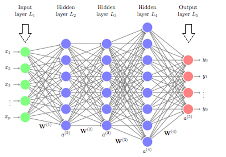
Traditional neural networks can’t do this, and it seems like a major shortcoming. For example, imagine you want to classify what kind of event is happening at every point in a movie. It’s unclear how a traditional neural network could use its reasoning about previous events in the film to inform later ones. Recurrent neural networks address this issue. They are networks with loops in them, allowing information to persist.

LSTM Networks

Long Short Term Memory networks — usually just called “LSTMs” — are a special kind of RNN, capable of learning long-term dependencies.LSTMs are explicitly designed to avoid the long-term dependency problem. All recurrent neural networks have the form of a chain of repeating modules of the neural networks. In standard RNNs, this repeating module will have a very simple structure, such as a single tanh layer.

The repeating module in an LSTM contains four interacting layers.

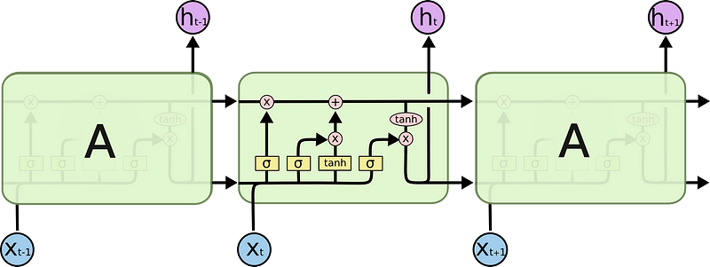
In the above diagram, yellow boxes denote the neural network layer, Pink circle denote Pointwise Operation, and arrows mention the Transfer, copy. Each line carries an entire vector, from the output of one node to the inputs of others. The pink circles represent pointwise operations, like vector addition, while the yellow boxes are learned neural network layers. Lines merging denote concatenation, while a line forking denotes its content being copied and the copies going to different locations. The key to LSTMs is the cell state, the horizontal line running through the top of the diagram. The cell state is kind of like a conveyor belt. It runs straight down the entire chain, with only some minor linear interactions. It’s very easy for information to just flow along with it unchanged.

The LSTM does have the ability to remove or add information to the cell state, carefully regulated by structures called gates. Gates are a way to optionally let information through. They are composed out of a sigmoid neural net layer and a pointwise multiplication operation. The sigmoid layer outputs numbers between zero and one, describing how much of each component should be let through. A value of zero means “let nothing through,” while a value of one means “let everything through!”

An LSTM has three of these gates, to protect and control the cell state.

---

Now From the above part, we can go through some ideas of the LSTM neural networks. So next move on to the Coding part. Here we choose python as the programming language using the following libraries.

import datetime, warnings, scipy 
import pandas as pd
import numpy as np
import seaborn as sns
import matplotlib as mpl
import matplotlib.pyplot as plt
from IPython.core.interactiveshell import InteractiveShell
import math
from keras.models import Sequential
from keras.layers import Dense
from keras.layers import LSTM
from sklearn.preprocessing import MinMaxScaler, StandardScaler
from sklearn.metrics import mean_squared_error

After importing the libraries then move to the data importing a part of the algorithm.

df = pd.read_csv('Data.csv', sep=' ')

So after importing the data the main process of the algorithm comes next. The calculation part for the quantile from each attribute. The following code snippet tells how the calculation was done.

def calculate_quantile (i, df2):
    Q1 = df2[[i]].quantile(0.25)[0]
    Q3 = df2[[i]].quantile(0.75)[0]
    IQR = Q3 - Q1
    min = df2[[i]].min()[0]
    max = df2[[i]].max()[0]
    min_IQR = Q1 - 1.5*IQR
    max_IQR = Q3 + 1.5*IQR
    
    return Q1, Q3, min, max, min_IQR, max_IQR

# delete first and last rows to avoid missing value extrapolation
df2.drop(index=[df2.index[0], df2.index[df2.shape[0]-1]], inplace=True)

# find and interpolate the outliers
for i in df2.columns:
    print('\nAttribute-',i,':')
    Q1, Q3, min, max, min_IQR, max_IQR = calculate_quantile(i, df2)
    print('Q1 = %.2f' % Q1)
    print('Q3 = %.2f' % Q3)
    print('min IQR = %.2f' % min_IQR)
    print('max IQR = %.2f' % max_IQR)
    if (min < min_IQR):
        print('Low outlier = %.2f' % min)
    if (max > max_IQR):
        print('High outlier= %.2f' % max)
    
    def convert_nan (x, max_IQR=max_IQR, min_IQR=min_IQR):
        if ((x > max_IQR) | (x < min_IQR)):
            x = np.nan
        else:
            x = x
        return x

def convert_nan_HUM (x, max_IQR=100.0, min_IQR=min_IQR):
        if ((x > max_IQR) | (x < min_IQR)):
            x = np.nan
        else:
            x = x
        return x
    
    if (i == 'HUM'):
        df2[i] = df2[i].map(convert_nan_HUM)
        df2[i] = df2[i].interpolate(method='linear')
    if (i != 'HUM'):
        df2[i] = df2[i].map(convert_nan)
        df2[i] = df2[i].interpolate(method='linear')
    
    if (len(df2[df2[i].isnull()][i]) == 0):

After the calculation then move to the next part which most important part of here the prediction part. So for this step, the data will split into some stages. Here we split the data 75% for training and 25% for testing.

train_size = int(len(dataset) * 0.75)
test_size = len(dataset) - train_size
train, test = dataset[0:train_size,:], dataset[train_size:len(dataset),:]
print(len(train), len(test))

After doing that, Now the LSTM neural network will create. Following is how the LSTM neural network was made.

model = Sequential()
model.add(LSTM(4, input_shape=(1, look_back)))
model.add(Dense(1))
model.compile(loss='mean_squared_error', optimizer='adam')
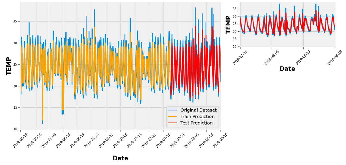
model.fit(trainX, trainY, epochs=1500, batch_size=32, verbose=2)

After creating a neural network all the prediction work is done. Now the results will tell how good was the prediction. Here is some example that I have done to analyze the temperature.

# shift train predictions for plotting
trainPredictPlot = np.empty_like(dataset)
trainPredictPlot[:, :] = np.nan
trainPredictPlot[look_back:len(trainPredict)+look_back, :] = trainPredict

# shift test predictions for plotting
testPredictPlot = np.empty_like(dataset)
testPredictPlot[:, :] = np.nan
testPredictPlot[len(trainPredict)+(look_back*2)+1:len(dataset)-1, :] = testPredict

# plot original dataset and predictions
time_axis = np.linspace(0, dataset.shape[0]-1, 15)
time_axis = np.array([int(i) for i in time_axis])
time_axisLab = np.array(df2.index, dtype='datetime64[D]')

fig = plt.figure()
ax = fig.add_axes([0, 0, 2.1, 2])
ax.plot(np.expm1(dataset), label='Original Dataset')
ax.plot(trainPredictPlot, color='orange', label='Train Prediction')
ax.plot(testPredictPlot, color='red', label='Test Prediction')
ax.set_xticks(time_axis)
ax.set_xticklabels(time_axisLab[time_axis], rotation=45)
ax.set_xlabel('\nDate', fontsize=27, fontweight='bold')
ax.set_ylabel('TEMP', fontsize=27, fontweight='bold')
ax.legend(loc='best', prop= {'size':20})
ax.tick_params(size=10, labelsize=15)
ax.set_xlim([-1,1735])

ax1 = fig.add_axes([2.3, 1.3, 1, 0.7])
ax1.plot(np.expm1(dataset), label='Original Dataset')
ax1.plot(testPredictPlot, color='red', label='Test Prediction')
ax1.set_xticks(time_axis)
ax1.set_xticklabels(time_axisLab[time_axis], rotation=45)
ax1.set_xlabel('Date', fontsize=27, fontweight='bold')
ax1.set_ylabel('TEMP', fontsize=27, fontweight='bold')
ax1.tick_params(size=10, labelsize=15)
ax1.set_xlim([1360,1735]);

Here is the output of it

The output of the temperature Prediction

Conclusion

From these code snippets, we can train the data and get an approximately 95% accurate model from the neural network using LSTM. In my last story, I was trying to predict the weather using Linear regression. From that, I got 93% accuracy. So, I'm still working get as more accuracy as possible for implement the successful neural network for the Air Quality prediction